
Remote Sensing: Description of Modules
Import Satellite Data
Satellite data can be imported here. Once the file is selected, the user can select which band to import. In addition, a conversion from UTM to SUTM is available.
This imports include:
ASTER data; note that this is the data as obtained from https://earthdata.nasa.gov. It can either be in .hdf format or imported as a zip file containing GeoTIFF images.
Landsat data; note that this is the data as obtained from https://earthexplorer.usgs.gov. It can either be in L*.tar.gz format or extracted, with a _MTL.txt and GeoTIFF files.
Sentinel 2 data; note that this is the data as obtained from https://earthexplorer.usgs.gov. It is the extracted directory, with an appropriate xml file (e.g. MTD_MSIL2A.xml).
MODIS data.
Hyperion L1T data.
WorldView Tile data; the tiles will be merged into a single dataset.
ASTER Global Emissivity data.
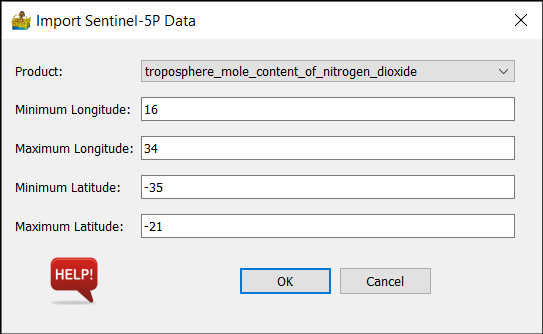
Import Sentinel 5-P
Sentinel 5-P data is imported here, but unlike other imports, this converts data to a vector data format, from where it can be exported to a shapefile using the context menu. It accepts .nc data. This import also allows the user to cut the data according to a bounding box. The options are:
Product - Relevant product contained in the .nc file
Minimum Longitude
Maximum Longitude
Minimum Latitude
Maximum Latitude
Create Batch List
This option allows the user to flag a directory of remote sensing data for use in other remote sensing modules that support batch processing. Note that it only imports metadata, and not band data. The user must select a directory as input. The options are similar to the regular satellite data import.
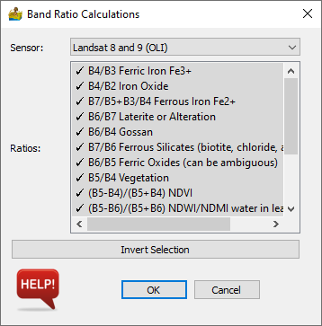
Calculate Band Ratios
This module allows the user to calculate ratios from a list of standard ratios found in the literature (Kalinowski and Oliver, 2004, Van der Meer et al 2014). It takes as input either a standard import of remote sensing data, or input from a batch list. The user must select the relevant satellite and confirm which ratios are needed. Ratios are automatically exported to new subdirectory names ‘ratio’.
Options:
Sensor - satellite sensor to base ratios on.
Ratios - selection for ratios available for the chosen sensor.
Invert selection - convenience button to invert the condition indices selection.
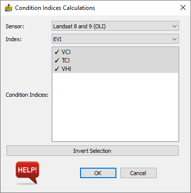
Calculate Condition Indices
This module allows the user to calculate condition indices such as TCI, VCI and VHI using indexes such as EVI, NDVI and MSAVI2. It requires as input two or more datasets over the same area, defined as a batch file list.
Options:
Sensor - this is the satellite sensor being used. Depending on the sensor, different indices will result.
Index - This can be EVI, NDVI or MSAVI2
Condition Indices - A list of indices to calculate
Invert selection - convenience button to invert the condition indices selection.
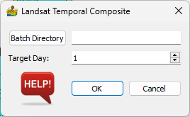
Landsat Temporal Composite
This module creates a temporal composite from a list of Landsat scenes. The aim is to substitute data from multiple scenes over areas with clouds.
Options:
Batch Directory - This is a directory where all the eligible scenes can be found
Target Day - This is the optimal Julian day for the scenes. It can be the mean day, or the day of the best scene. Scenes closest to this day will be given preference.
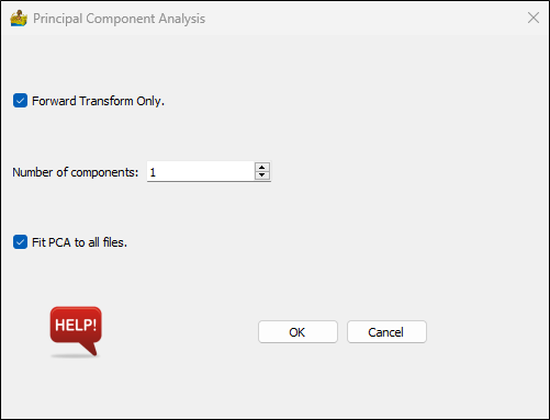
Principal Component Analysis
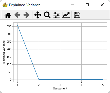
This module performs Principal Component Analysis (PCA) on data, with the aim of performing noise filtering. Upon completion of the calculation, a graph of explained variance is displayed, which can be used to assist in defining the optimal number of components for filtering.
The PCA module is also capable of accepting raster lists, so that batch PCA can be performed. In such a case, the user has the option to fit the PCA model to all files first, before translating the data to PCA space. This allows adjacent datasets to be mosaiced seamlessly, because the same model is applied to all input data.
Options:
Forward Transform Only - This outputs the forward transformed data with a preset number of components.
Number of components - Number of components used.
Fit PCA to all files - used to obtain a common PCA model over a number of files
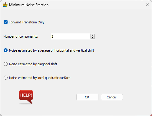
Minimum Noise Fraction
This module performs Minimum Noise Fraction (MNF) on data, with the aim of performing noise filtering. Upon completion of the calculation, a graph of explained variance is displayed, which can be used to assist in defining the optimal number of components for filtering.
Options:
Forward Transform Only - This outputs the forward transformed data with the specified number of components.
Number of components - Number of components used.
Noise estimated by average horizontal and vertical shift - This is the noise estimation as performed in ENVI.
Noise estimated by diagonal shift.
Noise estimated by local quadratic surface - Option recommended by Berman et al (2012), but slower.
Hyperspectral Imaging
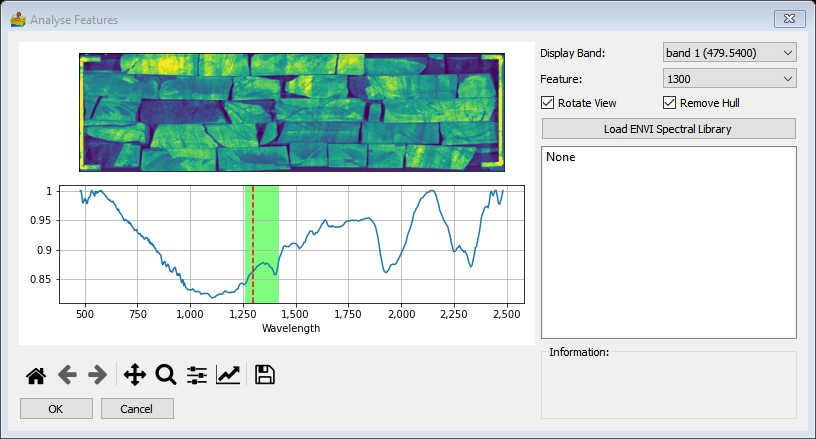
Analyse Spectra
This module allows for a user to select a spectrum from a dataset, and compare it with library spectra. Different features can be highlighted, and a hull can be removed from the spectrum. This tool is essentially a viewer, allowing for the user to strategize interpretation strategies.
Options are:
Display band – choice of which data wavelength to display.
Feature – highlight a standard spectral feature.
Rotate view – Allows a dataset to be rotated for display purposes.
Remove hull – allows for the hull removed representation of a spectrum.
Load ENVI spectral library. This can be any spectral library in ENVI spectral library format. The user then chooses the appropriate reference spectrum to compare with.
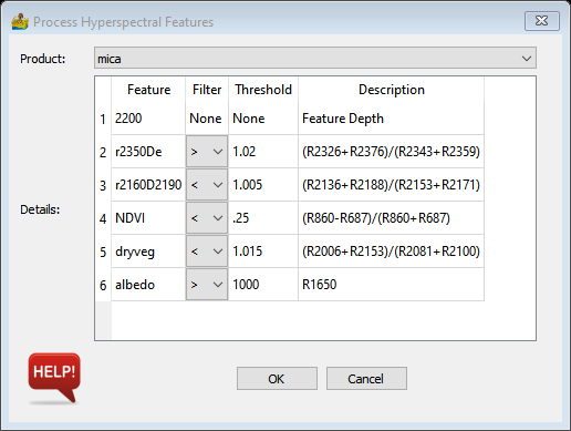
Process Features
This module takes as input hyperspectral data, and allows for a standard set of feature definitions to be calculated (Haest et al. 2012). Currently this includes mica, spectate, kaolin, chlorine, epidote and ferrous iron. Once a product is selected, the details of the various datasets which make up the calculation are shown on a table, including feature name, filter, threshold and description. The user is able to alter details such as the respective dataset threshold.
Options are:
Product - includes mica, spectate, kaolin, chlorine, epidote and ferrous iron.
Details - including feature name, filter, threshold and description. The user is able to alter the respective dataset threshold.
Change Detection
Change detection is an important technique used in the analysis of remote sensing data. Ordinarily, satellite data has a fixed number of bands (between 4 and 12 on average). These bands represent a light spectrum and can be utilised to study various terrestrial phenomena, from vegetation to minerals. The limits of the data are normally due to the number of bands in the data. One way to overcome this is to examine the temporal dimensions of the data. By studying the change in the data across multiple scenes, we can leverage more information.
Change detection relies on the changing nature of the earth. This can be from extreme environmental disasters such as fires and landslides, or as simple as studying the effect a seasonal change has on the target being studied.
This includes: 1) Landslides. 2) Environmental studies. 3) Land use and land cover. 4) Mineral outcrop (by using change detection as a process of elimination).
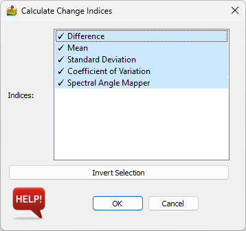
Calculate Change Indices
Change Detection Indices give a measure of change in an area. The input to this module is a list of datasets loaded using the batch importer. Each dataset must also have an associated date. The import tool for satellite scenes should assign a date automatically, but should a manual date need to be assigned, this can be done within the metadata context menu. A variety of change indices can be calculated:
Indices:
Difference - calculates the difference between two dates.
Mean - average pixel value image over all dates.
Standard Deviation - shows pixel variation though standard deviation.
Coefficient of Variation - measure of variation, taking mean into account.
Spectral Angle Mapper - find spectral angle between two scenes.
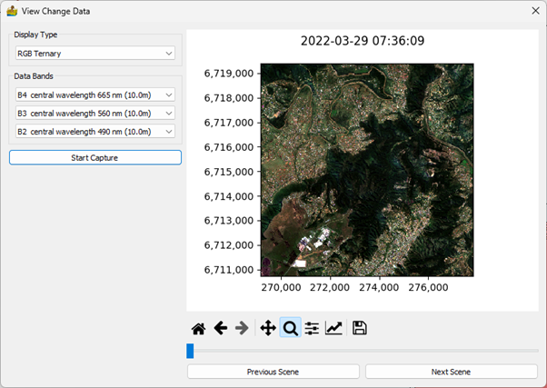
View Change Data
The visualisation of change is an obvious need for change detection. Often an end user wishes to see the scenes in sequence, rather than an index. As such a viewer is needed for this. The viewer requires only a batch list, coupled with associated dates for each scene. The viewer loads in the scene at a reduced resolution, suitable for a windows display. This increases speed, with the relevant section of the scene being reloaded upon zooming in. Because this viewer is dependent on reading constantly off a disk, slow image data formats are not supported. To optimise this, the viewer requires the data to be in GeoTIFF format. The main display also shows the date and time stamp for the scene.
The viewer options are:
Display type: sets the image to be displayed, whether single band or ternary.
Data bands: used to set each band to be displayed.
Start capture: The scenes can be exported to a GIF image, at the current resolution and zoom.
Previous and Next buttons: used to select the scene to be displayed.
Scroll bar – used to select the scene to be displayed.