

Hyperspectral Imaging#
The Hyperspectral Imaging module provides functions to analyse and process hyperspectral data. The imagery can be from a satellite, airborne survey or core scanner.
Analyse Spectra#
This module allows for a user to select a spectrum from a dataset and compare it with library spectra. Different features can be highlighted, and a hull can be removed from the spectrum. This tool is essentially a viewer, allowing for the user to strategize interpretation strategies. The dataset that will be analysed must be projected. The interface has the following aspects:
Image display - A single band or a true colour image can be displayed. Click on the image to show die spectral graph at that point.
Spectral graph - The spectrum at the point selected in the image is shown in blue. A library spectrum can be overlain and will be orange.
Display options - Discussed separately below.
Standard image display settings that allow the user to zoom into specific areas of the image, move the zoomed in area around, return to the full image, save the image with the colour bar, etc
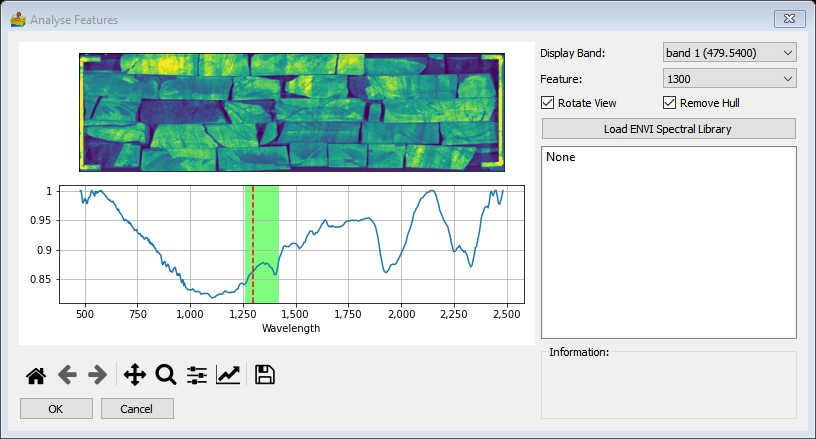
Analyse Spectra interface#
The display options are:
Display Band - Choice of which data wavelength to display.
Feature - Highlight a standard spectral feature on the spectral graph. The features are associated with typical absorption features for certain minerals and mineral groups (Laukamp et al., 2021; Haest et al., 2012):
900 - Ferric iron absorption feature (e.g. hematite)
1300 - Ferrous iron (e.g. magnetite)
1550 - Epidote
1760 - Sulphates (e.g. gypsum, alunite)
2080 - Pyrophyllite, topaz, talc
2200 - White micas, smectite
2250 - Chlorite, epidote, biotite
2290 - Ca-amphiboles, talc
2330 - Chlorite, carbonate
2390 - Amphiboles
True Colour Ternary - Select this to display a ternary image instead of a single band image.
Remove Hull - Allows for the hull removed representation of a spectrum.
Load Spectral Library - This can be any spectral library in ENVI spectral library format (SLI)or USGS SPECPR format. The user then chooses the appropriate reference spectrum to compare with.
Names of library spectra loaded in. Click on a name to display the spectrum in the spectral graph.
Current Spectrum Description – opens a description of the selected library spectrum.
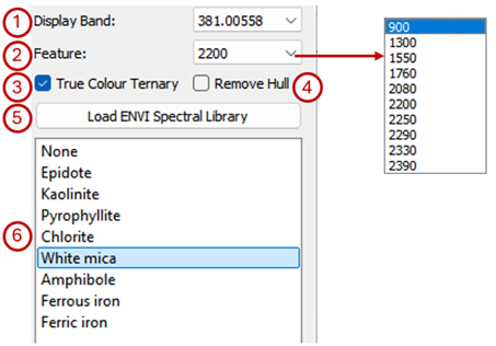
Display options on the Analyse Spectra interface.#
Process Features#
This module takes as input hyperspectral data (single dataset or batch list) and allows for a standard set of feature definitions to be calculated (Haest et al. 2012). These features are absorption features that are typically associated with certain minerals or mineral groups. Once a product is selected, the details of the various datasets which make up the calculation are shown in a table, including feature name, filter, threshold and description. The user can alter details such as the respective dataset thresholds.
The Process Features interface has the following options:
Product - A dropdown list of the minerals or mineral groups that can be detected:
Amphibole - The depth and wavelength (nm) of the 2390 nm feature are calculated.
Carbonate - The depth and wavelength (nm) of the 2320 nm feature are calculated
Chlorite - Features at 2250 nm and 2330 nm can be detected separately. The presence of both provides further information about the composition of the chlorite (Lypaczewski and Rivard, 2018). In both cases the feature depth and wavelength (nm) are calculated.
Epidote - The depth and wavelength (nm) of the 1550 nm feature are calculated.
Ferric iron - The depth and wavelength (nm) of the 900 nm feature are calculated. Note that the feature is usually broad making the wavelength difficult to calculate accurately.
Ferrous iron - This is a ratio and therefore no wavelength information is available.
Kaolin Group - The depth and wavelength (nm) of the 2200 nm feature are calculated.
Pyrophyllite - The depth and wavelength (nm) of the 2160 nm feature are calculated.
Smectite - The depth and wavelength (nm) of the 2200 nm feature are calculated.
White micas - The depth and wavelength (nm) of the 2200 nm feature are calculated.
Details - The first line in the table shows the wavelength of the defining feature. If the feature name starts with an f, the feature depth and minimum wavelength are calculated. If it starts with an r, a ratio is calculated. The remainder of the lines in the tables details filters that are used to link the specific feature to a mineral or mineral group. The Filter can be < or > and the user can set the threshold at which a feature is detected. The figure below shows an example to show how these details are used to detect a mineral.
Filter Albedo and Vegetation - When this option is selected, albedo and vegetation will appear in the table, and their filter and threshold settings can be adjusted.
If the final product is a ratio, filter out values less than 1 - If this is selected only the pixels where the feature was detected will be kept.
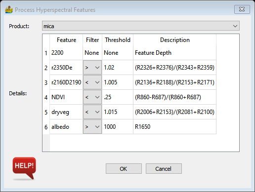
Process Features interface.#
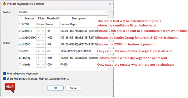
Example to show how the thresholds are used to ensure and absorption feature at 2200 nm exists and is indicative of smectite.#
After the calculation is done for a single dataset, the user can right click on the Process Features module and export the result using Export Raster Data. If a batch list was used to process multiple datasets, the results will be exported automatically with the feature name appended to the filename. For results with depth and wavelength a multiband raster will be stored.
References#
Haest, M., Cudahy, T., Laukamp, C. and Gregory, S. 2012. Quantitative mineralogy from infrared spectroscopic data. I. Validation of mineral abundance and composition scripts at the rocklea channel iron deposit in Western Australia. Economic Geology, 107, 209-228, https://doi.org/10.2113/econgeo.107.2.209.
Laukamp, C., Rodger, A., Legras, M., Lampinen, H., Lau, I.C., Pejcic, B., Stromberg, J., Francis, N. and Ramanaidou, E. 2021. Mineral physicochemistry underlying feature‐based extraction of mineral abundance and composition from shortwave, mid and thermal infrared reflectance spectra. Minerals, 11, https://doi.org/10.3390/min11040347.
Lypaczewski, P. and Rivard, B. 2018. Estimating the Mg# and AlVI content of biotite and chlorite from shortwave infrared reflectance spectroscopy: Predictive equations and recommendations for their use. International Journal of Applied Earth Observation and Geoinformation, 68, 116-126, https://doi.org/10.1016/j.jag.2018.02.003.