Classification Preparation

This case study uses clustering algorithms to integrate a digital elevation model (DEM) and airborne magnetic and radiometric data. The first vertical derivative of the magnetic data was calculated to enhance the shallow features.

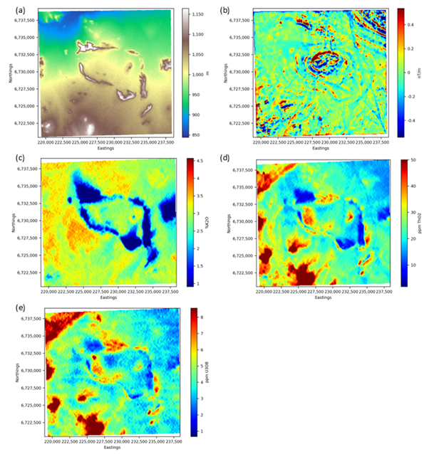
Potential input data for classification. (a) DEM; (b) First vertical derivative of the magnetic data; (c) Potassium data; (d) Equivalent thorium data; (e) Equivalent uranium data.

Data selection

It is important that datasets used in classification are not highly correlated since this will bias the results towards the correlated data. This can be checked using correlation coefficients. The datasets must first be merged into a single multiband dataset.

With the exception of equivalent thorium (eTh) and equivalent uranium (eU), the correlation coefficients are below 50%. The 88% correlation between eTh and eU means that only one of these datasets must be used. Since eTh is less noisy than eU it will be used.

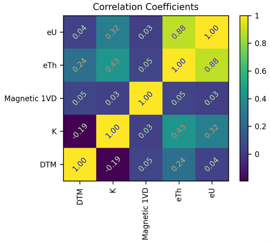
Correlation coefficients between the datasets shown in Figure 194.

Data preparation

Step 1: Ensure all the datasets are in the same projection

To check the projection of each dataset, look at its metadata. If necessary, reproject the data.

Step 2: See if the datasets need to be smoothed to remove high frequency noise

Datasets may contain high frequency noise that will affect the classification results. Radiometric data are particularly prone to this and often have a speckled appearance in the example data this is visible in the potassium data. A 2D mean smoothing filter using a disk window with a radius of three cells adequately removed the noise.

Step 3: Investigate the distributions of the input data for normality

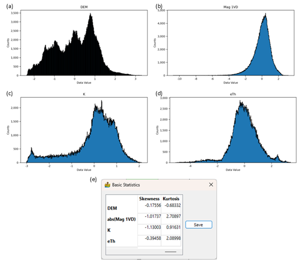
The statistical methods used in the classification algorithms work best on data with normal distributions. Look at each dataset’s histogram to establish its distribution. The Basic Statistics table also gives information on the skewness and kurtosis of the distribution. A normal distribution has a kurtosis of three and zero skewness.

The example data do not have normal distributions. The DEM’s distribution is flat and wide with short tails which results in a negative kurtosis and low skewness values. In contrast the magnetic derivative data have very high kurtosis which indicates a sharp peak with long tails. The tails are almost symmetric but slightly skewed to the right. Both radiometric datasets have highly skewed distributions. Potassium’s distribution is left-skewed while eTh has a right-skewed distribution.

Data can be transformed to have a distribution approximating a normal distribution. The simplest transformation is to calculate the logarithm of a dataset. This can be done using the Equation Editor. The user can test the natural logarithm (base e) and the decadic logarithm (base 10) to see which gives the best result. If the distribution is left-skewed the data can either be squared, its exponential can be calculated, or it can be reflected (subtract each value from the maximum and add 1) and then transformed using the logarithm. In this case the data should be reflected back after the logarithmic transformation (Osborne, 2002).

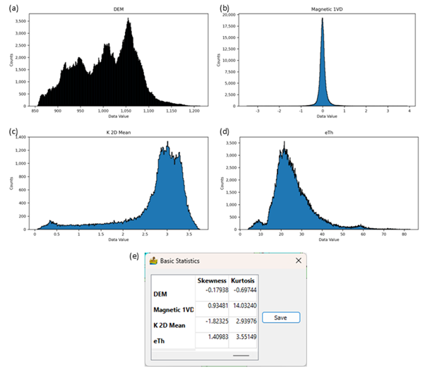
Histograms of the input datasets. (a) DEM; (b) First vertical derivative of the magnetic data; (c) Smoothed potassium data; (d) Equivalent thorium data; (e) Skewness and kurtosis for the distributions.

The dipolar nature of magnetic data presents another challenge. A positive and negative anomaly is linked to the same source but will be considered as two separate bodies during cluster analysis. One option is to reduce the data to the pole, but the presence of remanent magnetisation will diminish the effectiveness of this method. Paasche and Eberle (2009) addressed this problem by calculating the absolute value of the magnetic first vertical derivative. This results in a very skewed distribution. .. figure:: _images/tutclass4.png

Histogram and statistics of the absolute value of the magnetic first vertical derivative data.

Step 4: Transform the data as required to approximate normal distributions

If the same transformation will be applied to all datasets, the individual datasets can first be merged/stacked into a single multiband dataset and the transformation applied in a single step. However, at times different transformations need to be applied (as in our example case) and it is simpler to transform each dataset separately.

For this example, the DEM will not be transformed since none of the transformations influenced the distribution. The absolute value of the magnetic data and eTh were transformed using the decadal logarithm. The histograms for the transformed data are less skewed and therefore better approximations to a normal distribution. Since the potassium data is left-skewed an exponential transform was applied but the result was a histogram with two peaks. The data were then reflected and the decadal logarithm calculated, after which the data were reflected back to restore the original order. The left tail remained but is somewhat shorter than for the original data.

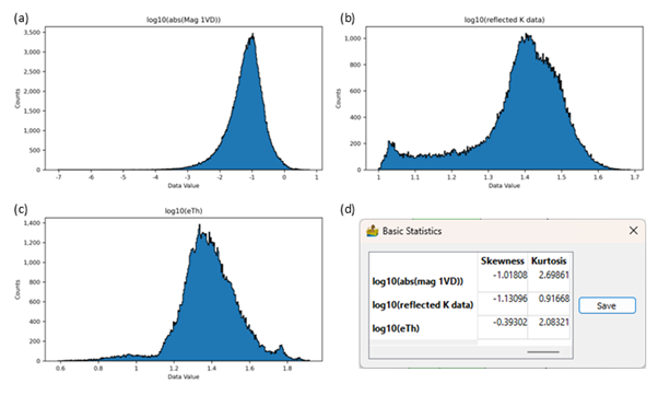
Histograms of the transformed datasets. (a) First vertical derivative of the magnetic data; (b) Potassium data; (c) Equivalent thorium data; (d) Skewness and kurtosis for the distributions.

Step 5: Combine all the datasets into a multiband dataset

For the classification routines the data must be in a single multiband dataset. Use Layer Stack and Resampling to do this.

Step 6: Normalise the data

It is important to normalise the data prior to classification to ensure that the data values of the different datasets fall in the same range. If this is not done, the results will be biased towards datasets with larger values. The example data were normalised using a mean of zero and standard deviation of 1. This dataset was then stored.

Histograms of the normalised datasets. (a) DEM; (b) Absolute value of the first vertical derivative of the magnetic data; (c) Potassium data; (d) Equivalent thorium data; (e) Skewness and kurtosis for the distributions.

The next figure shows the whole data preparation workflow in PyGMI.

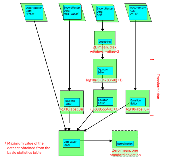
Data preparation workflow in PyGMI. Red text indicates the options selected for a module and user inputs.

References

Osborne, J.W. 2002. Notes on the Use of Data Transformation. Practical Assessment, Research & Evaluation, 8.

Paasche, H. and Eberle, D.G. 2009. Rapid integration of large airborne geophysical data suites using a fuzzy partitioning cluster algorithm: a tool for geological mapping and mineral exploration targeting. Exploration Geophysics, 40, 277–287, https://doi.org/10.1071/EG08028.